I started programming at the age of 15 (I was in High School specialized in CS), then I was studying Mathematics and, after that, worked for 4 years as SE. Finally, I was doing Ph.D. in Computational Physics. So at the beginning of my preparation process, I already forgot algorithms classes from my high school but I knew quite well several programming languages.
I started my preparation more than a year before having interviews with target companies. The plan was to spend around 2h a day on this task. At the first step, I read the whole Cormen (March’16-September’16). I solved most of the exercises and implemented all the algorithms except those which are irrelevant for the interview like FFT. To practice, I solved around 250 problems from the book “Elements of programming interview”. I typically read one chapter per week and solved 1-2 problems per day. In addition, I was solving problems from Leetcode (June’16-July17). At the beginning, I was solving a few easy per week. During the second step, I was reading topcoder algorithms tutorials and solving some problems listed there. At that time, I was solving 1-2 problems from leetcode a day, sometimes participating in the contests. During the third preparation step, I solved around 100 problems on leetcode for 3 weeks (it was right before Google telephone interview). The final preparation step (preparation for Google onside) was solving contest per day (topcoder, hackerrank, hackerearth), plus 2 problems per day on a whiteboard.
Looking back I see quite many mistakes which did my preparation more time consuming than it could be. In particular, I should have concentrated more on the goal - develop skills in problem-solving. So there is no need to spend so much time on Cormen. Participate more in contests from the beginning, and others.
Thus, a posteriori, I would give build my preparation strategy on the following principles:
1) Use small iterations while preparing.
2) Find and use metrics for performance to evaluate your progress and weak points.
3) Read books/blogs about algorithms only by demand. First check out e-maxx.ru/algo/, which provides a brief algorithm explanation, and only after that read Cormen in case if you still don’t understand it.
4) Participate in all the contests you can find.
5) Gradually increase the complexity, does not makes sense to solve div1C if you are not comfortable with div1A.
More specifically, I would split the whole process into 3 weeks iterations. Before starting each iteration, you evaluate your strength and weaknesses using well-defined metrics. My metrics were:
a) time to solution: for easy/medium/hard,
b) accuracy of solution: how many times you need to run the code before submitting to find out all bugs, how many test cases it passes
c) whiteboard: how good is your explanation
d) mental stamina: do you manage to solve problems for several hours in a row (in contests, for instance)?
I would recommend to take problems from archives of topcoder, codeforces, codejam, hackerearth, hackerrrank or participate in a competition if at that date there is one. To practice standard interview problems, use leetcode - it has so-called “mock-up” mode which shows your time-to-solution and distribution of other users. Ideally, you need to solve 3 problems a day which corresponds to your current level.
1.1 Cover simple ad hoc problems, which do not require any algorithms knowledge. Plenty of them are on leetcode (easy), topcoder div2a, codeforces div2a or b. K
1.2 Study binary search. Check out topcoder tutorial, hackerearth tutorial. Also, you can find relevant problems there.
1.3 Checkout greedy algorithms. The same sources.
1.4 Cover simple dynamics. The same sources.
Achieve proficiency in basics. Solve problems on these topics on different resources. Key metrics: time to solution, an accuracy of solution. You must not do mistakes on these problems.
Cover the next topic (graph algorithms, more complicated dynamics, sweep line, combinatorics, etc). Practice problems for this topic. Also, solve random contests and, when you meet something you have no clue about, study this topic and practice. Evaluate your performance every several weeks.
Evaluate your weaknesses, increase the complexity of the problems you solve. Go to step 3.
We used Dissipative Particle Dynamics for the fluid modeling and fluid-structure interactions. The solid walls were modeled using Signed Distance Function. We employed validated red blood cell membrane model which takes into account both elastic and viscous terms.
Although uDeviceX is not the first package where mentioned models were used, it is the most computationally efficient software and the first available online. Our work is among the finalist of the Gordon Bell Award 2015. In particular, we demonstrated perfect weak scalability on the whole Titan (18,688 KX20 GPU nodes) and good strong scalability on Piz Daint. Details about software, test cases, and performance results are published in ACM SC’15 Proceedings.
A recently published video of some simulations in microfluidics using our software:
The authors order corresponds to the contribution to the visualization. Mitsuba was used for rendering.
]]>Recently I came across an amazing paper “Robust fairing via Conformal Curvate flow” by K. Crane et al. at SIGGRAH 2013 and decided to reproduce the results. The basic idea of the approach is in usage of the principal curvatures instead of vertex coordinate itself for the solution of PDE. Roughly speaking, at each iteration for every vertex the curvature is computed, than modified according to the chosen PDE, and, finally, a new position is restored out of the curvature. So for instance, you want to edit your surface or curve using Willmore flow, traditionally it is evaluated in terms of positions of vertecies themself, it involves spatial dirivatives, Laplace-Beltrami operator depending on positions. Thus the implementation is complicated and the numerical scheme requires small time steps to converge. By constrast, reformulataion of the problem in terms of curvature gives a very simple numerical scheme, which works with much bigger time steps (in current work 108 times bigger). In addition to that, this reformulation allows to preserve desired properties of the manifold (e.g. length, angle).
Crane et. al. created a general framework and applied it to 1D manifolds (curves) and 2D manifolds (surfaces). I reproduced results only for the 1D case, since 2D is much more time consuming - working with group of quaternions, half-densities, and dirac operator - is too much for a hobby project.
Fist of all, I would recommend to read materals for the course in Discrete Differential Geometry provided by K. Crane. There one might find a very detailed explanation of the length-preserving curvature flow in the curvature space, described in the paper. In addition to that, there are formulas for the standard Willmore flow for the curve and nice scatches. You also might find some details in Crane’s dissertation, but primarily if you want to implement a 3D case (there is a discretization of the Dirac operator, explanation of the exterior calculus on quaternions, many proofs used for the theorems used in the paper, etc). At the moment of the writing this post, authors of the paper didn’t shared their implementation for the isometric curvature flow, so I implemented it by myself (but sometimes asking K.Crane about some details, he was very helful).
The text will be structures as follows. First, I will give basic definitions. Than I will describe the approach by Crane et al. and show some simulation results on the models provided by K. Crane. Finally, I will briefly describe a standard Willmore flow and show simulation result for comparison.
Definition: , where M - (n-1)-manifold with boundary is called immersion if is injective map.
Definition: let f be an immersion of a manifold M into Euclidean space, and suppose that E is a real-valued function of f. Then a curvature flow is the solution to the partial differential equation . We call E energy.
Common choices of energies are the Dirichlet energy and the Willmore energy , where H is a mean curvature (for M without border). Further, we will work with Willmore energy. Further, Willmore energy is employed.
It is easy to show that energies can be rewritten as and , where denotes inner product in . denotes Laplace-Beltrami operator, note that it itself depends on the immersion f. It leads to non-linearity of the corresponding flow equations formulated in terms of immersions.
In their work Crane et al. created an implementation for both 1D and 2D manifold. I will consider Willmore flow only curves. Let describe the geometry of the curve via an immersion for interval .
We will work with two definitions of energies - one to get a Willmore flow using a standard approach , another one is used for the conformal Willmore flow . The difference between them is in the second case it is a function of the curvature rather than immersion f. It allows to solve simpler PDE, having a better convergence and also restore positions in a way that preserves desired properties.
First consider the solution using standard approach. Let introduce notation which will be used further: is a tangent vector, is curvature, denote Hodge star, means a dual edge, 
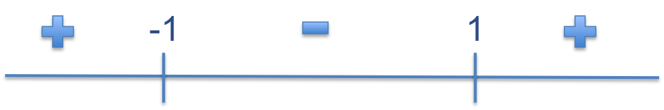
is an exterior angle for the dual edge, Hodge star on primal 0-form is given by . We will use the fact that to define for the discrete curves: .
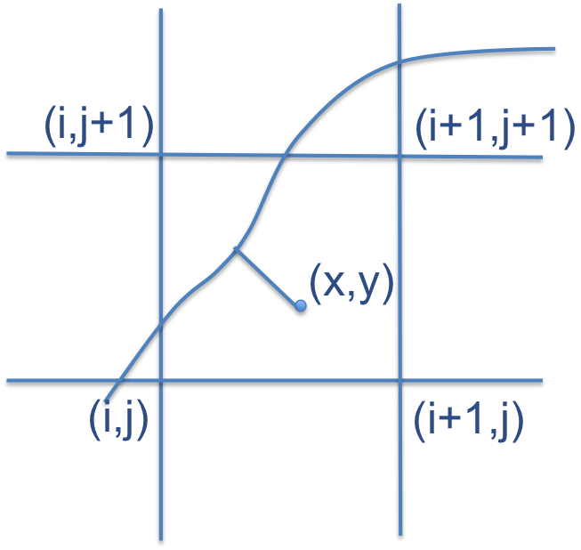
Another important notation is a gradient with respect to the vertex p denoted by - consider a triangle with a fixed basement and a vertex opposite to the basement. Without goint into details the gradient will be written as follows:
A scheme of the proof might be found on the DDG course page. In order to implement the flow, one shall implement these formulas. In my case these formulas didn’t work as is, I added condition that if the angle is 0, than the gradient is 0, I also use absolute value of the angle. Finally, I suspect that there is a mistake somewhere in the gradient for the previous and the next vertices. However, the goal of having this method here is demonstrating how cumbersome it is and also to demonstrate that theis flow is much slower than the flow in curvature space. So since these formulas work for the square and bunny, it is enough.
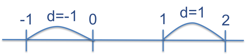
At the end I would like to mention that the exterior angle should be in range .
It might be computed like that: atan2(u.x * v.y - v.x * u.y, dot(u, v))
. Curvature for this point is then just .
If we consider an energy instead of then the resulting flow is much simpler and works for bigger timesteps.
First give a continuum formulation. The gradient with respect to inner product is , thus the gradient flow is . After modifying the curvature we can restore the angle by integrating the curvature . Having we can calculate tangent vector and from that we can restore immersion .
The discretization is the following:
In addition, we must take into account that the curve is closed, e.g. and . Without providing a proof - it is equavalent to having the following conditions: . For the descrete case, one need to work in a space where n is the number of points on the curve but with the inner product immersed by the function itself. It means that we need to create a diagonal mass matrix B where element on the diagonal are just and when computing inner product use it . The vectors we should orthogonalize are where anf are x and y components of positions. At the end, should be orthogonal to all other vectors.
The algorithm overview is presented below.
Note that the resulting flow is isometric by construction - we do that at two last steps.
The simulation results tell us that in case of the standard approach the biggest stable time step is while for Curvature flow in curvature space we have . So it is up to times bigger! Not suprisingly you will wait forever to obtain the flow using standard approach (several minutes) while Crane’s et al. approach propagates the curve in a second or so. 
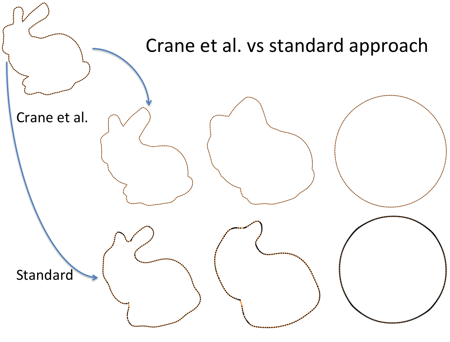
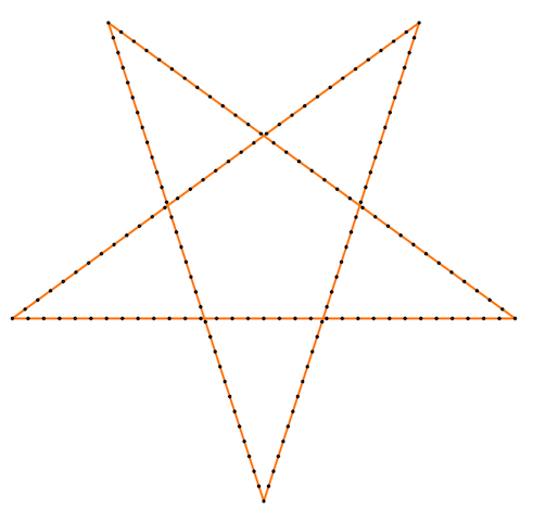
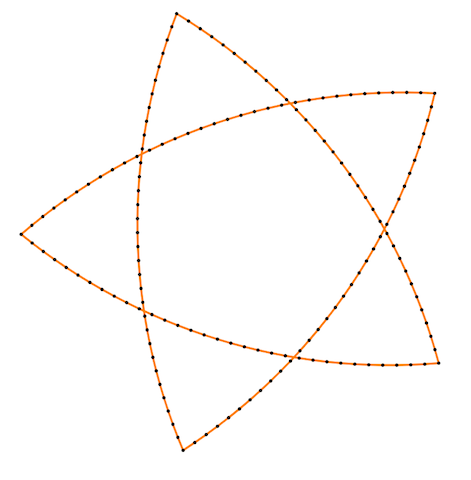
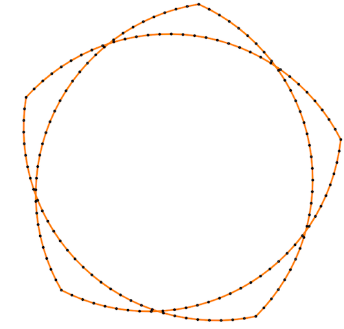
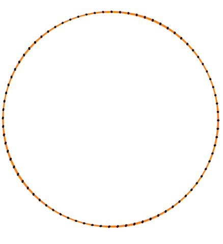
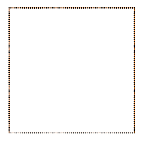
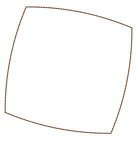
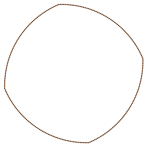
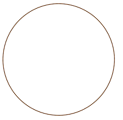
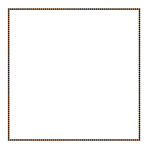
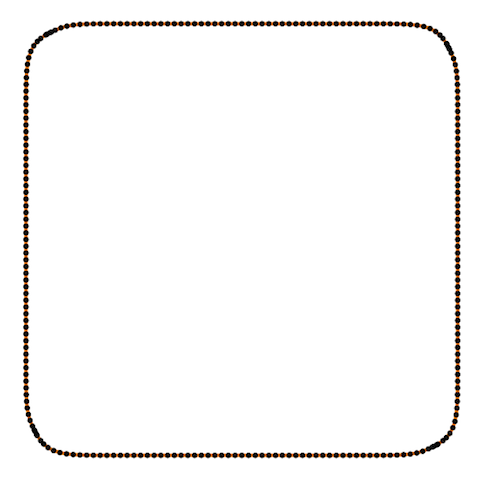
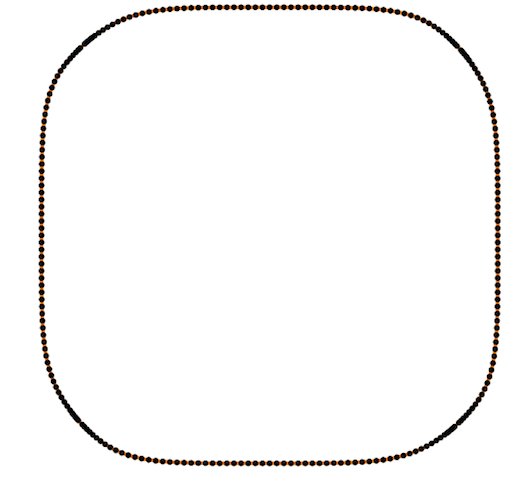
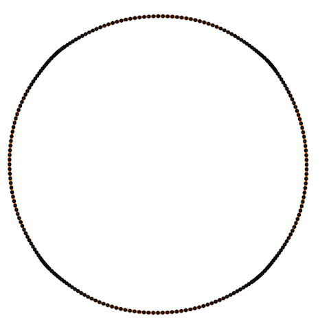
Also Crane’s et al. approach gives isometric flow, while standard doesn’t. It might be seen on the figure below - point are distributed uniformly in the first case, and not uniformly in other:
Finally, some more picture for the Isometric curvature flow:
And one more for the standard one:
Seam carving is an algorithm for content-aware image resizing, it was described in the paper by S. Avidan & A. Shamir. In contract to stretching, content-aware resizing allows to remove/add pixels which has less meaning while saving more important. Pictures below demonstrate this - original picture of the size 332x480 is on the top, the picture after applying seam carving (size is 272x400) is on the bottom
This algorithm is quite impressive so one may find a lot of articles describing it. Yet as I found most of the authors haven’t read the original paper and provide a very basic implementation. In this post I will describe the algorithm with all details as it was written by Avidan & Shamir. Yet I will write from the programmers point of view, without going into Math too deep. In addition to algorithms description, I also provide Matlab code.
For simplification, we will describe only reducing the size of the image. But enlarging process is very similar and described in the last section.
The idea is to remove content that has smaller meaning for the user (contain less information). We will call this information “energy”. Thus we need to introduce an energy function that would map a pixel into
energy value. For instance, we can use gradient of the pixel: . If a picture has 3 channels, just sum values of the energy in each channel. The Matlab code below demostates it. The imfilter
function just applies the mask to each pixel, so the result dI(i, j)/dx = I(i+1)-I(i-1)/dx where dx = 1.
1 2 3 4 5 6 7 8 9 10 11 |
|
Here is energy function:
If we delete pixels with minimum energy but random positions, we will get distorted picture. If we delete columns/rows with minimum energy, we will get artifacts. Here by column I mean {(i, j)| j is predefined}, row - {(i, j)| i is predefined}. The solution is to introduce a generalization of column/row (called seam
). Formally, let I is n x m image, then a vertical seam is , where x: [1,..,n] -> [1,..,m]. It means that a vertical seam is path from the top of the picture to the bottom such that the length of the path in pixels is width of the image, and for each seam element (i,j),
the next seam element can be only (i+1, j-1), (i+1, j), (i+1, j+1). Similarly, we can define a horizontal seam. Examples of seams are shown on the figure below in black:
We are looking for a seam with the minimum energy among all seams (in chosen dimension): . The way to find such an optimal way is by using dynamic programming:
Note that in Matlab code I had to represent seam as n x m bit matrix. If pixel is in the seam it is 0, otherwise 1.
1 2 3 4 5 6 7 8 9 10 11 12 13 14 15 16 17 18 19 20 21 22 23 24 25 26 27 28 29 30 31 32 33 34 35 36 37 |
|
In order to find a horizontal seam, just pass a transposed energy matrix to findOptSeam
.
Now we can compute seams and using the code below we can even remove them from an image:
1 2 3 4 5 6 7 8 9 10 11 12 13 14 15 16 17 |
|
It is already a good tool for reducing image in one dimension - just find and delete seam as many times as you need. But what if you need to reduce the size of the image in both directions? How to decide at every iteration whether it is better (in terms of energy minimization) to delete a column or a row? This problem is solved, again, using dynamic programming. Let n’ x m’ are desirable size of the image (n’ < n, m’ < m). We introduce a transport matrix T which defines for every n’ x m’ the cost of the optimal sequence of horizontal and vertical seam removal operations. It is more suitable to introduce r = n - n’ and c = m - m’ which defines number of horizontal and vertical removal operations. In addition to T we introduce a map of the size r x c TBM which specifies for every T(i, j) whether we came to this point using horizontal (0) or vertical (1) seam removal operation. Pseudocode is shown below:
1 2 3 4 5 6 7 8 9 10 11 12 13 14 15 16 17 18 19 20 21 22 23 24 25 26 27 28 29 30 31 32 33 34 35 36 |
|
And Matlab imeplementation:
1 2 3 4 5 6 7 8 9 10 11 12 13 14 15 16 17 18 19 20 21 22 23 24 25 26 27 28 29 30 31 32 33 34 35 36 37 38 39 40 41 42 43 44 45 46 47 48 49 50 51 52 53 54 55 56 57 58 59 60 61 62 63 64 65 66 67 |
|
In order to enlarge a picture, we compute k optimal seams for deleting but then, instead of deleting, copy average between neighbors:
1 2 3 4 5 6 7 8 9 10 11 12 13 14 15 16 17 18 19 20 21 22 23 24 25 |
|
The full code of the program is available here. Seam carving is also implemented in ImageMagick. So if you need a C++ implementation, check out ImageMagick code.
]]>From the high-level of view level-set method (further just level set) can be considered as geometry representation, in addition to polygonal meshes and NURBS. This geometry representation simplifies solution of some problems in Computational Geometry, physical based modeling in Computer Graphics. Although level sets were first used for geometry tracking in 80s by Osher and Sethian, the main development of this method took place in the end of 90s and during 2000s.
OpenVDB is a new library by DreamWorks which contains data structures and tools for work with three-dimensional grids. In particular, it contains tools to work with level sets. OpenVDB is a very new library, before this library there was only one well-developed library addressing level set - Field3D. Yet it didn’t fit my needs so I wrote levelset-light library for my needs.
In order to use OpenVDB you need to build it. In case if you use Mac OS the following post might be useful for you - OpenVDB build on MacOS. Pay attention to the tools vdb_print
and vdb_view
in the bin
folder in the OpenVDB installation directory. I will use these tools for visualization of the computation results so if you want to follow, check that they are working. In case if you are using Mac, you might have problems with vdb_view
because shader language version used inside is not supported by Mac. In order to fix it, have a look inside of this patch. One more comment before we start, if you are suffering from the long compilation time of the code which uses OpenVDB, check out this discussion.
Level set of an implicit function is a set of points where this function has a predefined value. For instance, lets consider a function . It describes a parabola which intersects axe x in two points -1 and 1, thus the set of points where f is equal to 0 (a predefined value, can be any number) is .
In practice, a level set function is usually constructed as a signed distance function. I.e. for a given surface and an arbitrary point, we define such a function as a signed distance from the point to the surface: if the point is outside the surface the function value is positive, if it is inside - negative, and, finally, 0 if it is on the surface.
Coming back to the example above, the surface is composed of two points in 1D space: {-1, 1}, all points which belongs segment (-1, 1) are inside our surface, other - outside. We want to construct a signed distance function so, in order to start, lets get an arbitrary point 2 which is outside of the surface. The distance from this point to the surface is, obviously, 1. It means that we cannot just use . For another point 0 the distance from the point to the surface is -1. As one might guess the signed distance function for our surface is .
1D space is not really interesting so lets move to 2D and construct a signed distance function for a circle with the center in the origin and radius R. Lets get an arbitrary point x = (x, y) outside the circle (vectors are in bold here and further). The distance from the origin to this point is basically . Thus the distance from the point to the surface is |x| - R.
In 3D space, where x=(x, y, z), the distance to the z-axis parallel cylinder surface is represented by the same function .
Following similar logic, one can write distance functions for other figures such as sphere, torus, cone, etc.
It is cool to have a new geometry representation for primitives but what if one wants to use something more complicated? E.g. surface which constructed by surfaces of two cylinders A and B. For simplicity, cylinders are z-axe oriented, so they are described by their centers and radiuses. For cylinder A, the center and the radius are denoted by , similar for cylinder B. Given an arbitrary point x outside interior of these figures, we have two distances from the cylinders: , and similar d_B. The cross-section of this two cylinder is shown below.
Because we want to have union of this two figures, we use as a value of the distance function for x. In case if x is interior part, min will be applied to negative values and, thus, pick up the biggest in the module. Thus the part of the surface, which is inside the union of two of them, will disappear.
Other set operations on level sets are represented below:
Union:
Intersection:
Complement:
Difference (A \ B):
Although a level set might be represented by a set of continuous level set functions and operations on them (similar to NURBS), in practice, the level set geometry is stored in a file as a grid. Every grid vertex stores the exact function value. Thus if we want to get the distance from an arbitrary point in the space to the surface, we use interpolation: find the cell of the grid to which this point belongs to and interpolate function value in this point. For instance, in 2D case for a point (x, y) we can compute a pair of indexes (i, j) which describes the cell for the point as shown on the picture below:
So lets create a level set of a cylinder with center in the origin and z-axis oriented. In order to do that, we need to specify the radius of the cylinder, the grid dimensions, and the voxel (cell of the grid) size.
Pay attention that in OpenVDB you have an index space for your grid and a world space. Index space for the grid is , note that index might be negative. If (i, j, k) is a point in the index space, then is the point in the world space, where is a vector of voxel sizes.
The code below creates a grid which contains floats, specifies bounding box of our level set in the index space, and pass everything to makeCylinder. For simplicity uniform grid is used so . In order to modify elements of the grid, accessor object is used. Inside, we have loop on all points in the grid where we compute value of the function. In order to use our grid further, we need to define interpolator which will be used with this grid. It is done by calling method setTransform
.
It is easy to see that makeCylinder
might be generalized by introducing additional argument of type std::function\<float (const Vec3d&)\> lsFunc
(in C++11) which allows to fill in a grid by any signed distance level set function.
1 2 3 4 5 6 7 8 9 10 11 12 13 14 15 16 17 18 19 20 21 22 23 24 25 26 27 28 29 30 31 32 33 34 35 36 37 38 39 40 41 42 43 |
|
After running this application, you should get something like that:
It is cool to be able to create and save a regular grid in the file. Yet there is one pitfall - the file containing simple cylinder is 2.67MB in size:
1 2 |
|
As you might guess there are a lot information in the grid which we are not interested in - all grid vertices which are far away from the surface . OpenVDB allows to store only points which are in vicinity of the surface. The code below demonstrates it.
1 2 3 4 5 6 7 8 9 10 11 12 13 14 15 16 17 18 19 20 21 22 23 24 25 26 27 28 29 30 31 32 33 34 35 36 37 38 39 40 41 42 |
|
For every point it saves a value in the grid only if . In the code, backgroundValue
specifies the module of this distance. Note, that the call of the method signedFloodFill()
propagates the sign from initialized grid points to the uninitialized, since the background value is set in the grid by module. signedFloodFill()
might be used on closed surfaces only, so I picked up a sphere instead of a cylinder.
If you run this code and use vdb_print to check out the information about grid you will get that the grid is 27x27x27 instead of 40x40x40.
For a more optimal code for sphere generation, check out openvdb/tools/LevelSetSphere.h
.
Reading the grid is straight forward, the code below demonstrates it. Pay attention how to use linear interpolator in order to find a value of the level set function for an arbitrary point. Venusstatue.vdb is available here.
1 2 3 4 5 6 7 8 9 10 11 12 13 14 15 16 17 18 19 20 21 |
|
In the next part I will write about more advanced things such as deforming level set surfaces using PDE.
If you have any questions / suggestions about this material or a collaboration idea regarding level sets / openvdb, feel free to contact me.
]]>1 2 3 4 5 6 7 |
|
If you need any support, please write to issues, click button “New Issue” and then add a proper label - bug or question. An alternative option is to write to my email (address is written in the About section of this blog).
UPD: Since I shared this tool, I’ve got many letters with questions. Primarily from students who are doing something with Kinect. The most questions are about building oni2avi, so below are some recomendations:
There are two ways of building openvdb - build it under Houdini environment (you need to install houdini) and the second way using macport(no need in Houdini,
this way is described in the post). In order to build openvdb using Houdini, go to Applications/Houdinimake
and everything should be built. Yet, you may have problems with vdb_view, they are fixed in the patch, have a look inside. If you use a newer version, you will have problems with the HDK’s boost which is 1.46. I just renamed the folder with boost in hdk and specified path to a more recent version. Just in case if you forgot, if you want to build openvdb with sudo
, you need to use sudo -E
instead in order to have all environment variables on place.
Now, how to build OpenVDB without using Houdini and with the modern gcc. First of all, you need to have macports installed, then I would recommend to install the latest gcc. After that install OpenVDB dependencies:
1 2 3 4 |
|
The only problem is to install optional package glfw
(download sources):
1 2 3 4 5 |
|
pkg-config libglfw.pc In order to simplify linkage of openvdb with glfw (it requires opengl and cocoa), do pkg-config in glwf home:
1 2 3 4 |
|
After that you need to set up paths to libraries and includes in Makefile in the openvdb directory. I made several modifications in the openvdb, all of them can be extracted from the patch: - modified Makefile - added boost-system-mt library, added dependencies for vdb_view and other changes - modified vdb_view code so it can work with OpenGL 2.1 and GLSL version 120 - modified one test which can not be compiled without a error in the gcc4.7.2
In order to apply patch:
1
|
|
When you are done, run make
, make install
in the OpenVDB src directory. You may try to run vdb_view from the bin
directory in the your openvdb installation path.
In order to do that, download on of the shapes from the openvdb site, for instance icosahedron and run:
1
|
|
The result should look like on the figure below:
Then you may run tests (it takes a lot of time so I would skip it).
When I did it, I found a error (testIO) which leads to program termination. The problem is in cpp-unit I use (1.12.1), to fix it comment call of CPPUNIT_ASSERT_NO_THROW
in the TestCoord.cc lines 120 and 123
.
When you will try to use your openvdb library you may have problem: dyld cannot find an image. To fix this problem you may write export DYLD_LIBRARY_PATH=$DYLD_LIBRARY_PATH:<path_to_your_openvdb_lib>
.
In the simplest case, the file consists of header section where it is needed to specify names of columns:
1
|
|
And so called “ZONE” section which consists of header and columns:
1 2 3 |
|
This format can be used for the velocity and density fields visualization. To obtain this data from the simulation, you need to use fix ave/spatial:
1
|
|
This fix writes data in lammps own data format which can not be read by tecplot by default. In order to simplify your life and avoid modifying output file by hands, I modified this fix a little bit so if the file has extension “tec”, fix writes in the tecplot data format. It is difficult to do in post processing script because tecplot requires information about bins in every direction. Replace you ave/spatial with fix_ave_spatial.h, fix_ave_spatial.cpp, build and run LAMMPS. In order to open “velprof.tec” in tecplot go File->Load DataFile -> TecPlot data loader. In the left panel choose “Contour” (pick up D column, it is density). Then on the same panel click on “Vector” and choose columns “VX”, “VY”, “VZ”. I usually use slices for visualisation, in order to have slice Click “Slices” on the left panel, then specify properties of your slices, then go Data->Extract->Current Slices… In Zone styles panel you may define which slices are visible and which ones are not. So at the end you might have picture like the following one:
In addition to that you may visualise your particles using tecplot. In order to do this, you need to use restart2data tool (lammps->tools), and then atom2plt script. The pipeline is the following:
1 2 |
|
After that you will have *.plt file which can be opened in TecPlot. If you domain is periodic and you see some long dark lines, cut in tecplot your data a bit. Note, that this code works only for molecular atom style and in 3D. If you need another configuration and changed mentioned code, I would be glad if you commit in corresponding git repository or send me a patch.
]]>Before doing something, check tools available on your system and pick up the newest one. To see available versions of Cray compiler:
1
|
|
If the most recent version is, for example, 8.1.2, load compiler and switch to the last version:
1 2 |
|
Then check and load perftools:
1 2 |
|
Now, build an application and instrument your executable with profilers stuff:
1 2 |
|
It will create a new executable lmp< machine name>+pat. Further, you need to use this executable for your job. If you use SLURM, write in your sbatch script something like that:
1
|
|
where -n 32 means that you use 32 nodes, the hardware performance counter experiment is defined by setting the environment variable PAT_RT_HWPC. More info about this option can be found a the end of the following. page. When you job is done, call pat_report:
1
|
|
This application will create a file with extension ap2. You can explore performance of your application in text editor
(vi
1
|
|
Note, that in order to use it you need to have xwindow installed on your local machine and when you connect to your cluster you need to specify that it can use your monitor (-Y option):
1
|
|
(1) Run LAMMPS with the following script
1 2 3 4 5 6 7 8 9 10 11 12 13 14 15 16 17 18 19 20 21 22 23 24 25 26 27 28 29 30 31 32 33 34 35 36 37 38 39 40 41 42 |
|
(2) Open vel-visc and copy in a separate document data for one time step.
(3) Open gnuplot, type:
1
|
|
The result should be something like:
(4) From analytical solution for the problem, it is known that . Where , p - is numeric density(3.0 in our case, determined by custom lattice), g is driving force (0.055), n - dynamic viscosity. In order to find alpha we will use gnuplot’s fit command. As you might see on the Figure above, there are 2 parabolas. I pick the left one, so the analytical solution look like . Then type
1 2 3 |
|
The result should be , thus viscosity n=2.68 in DPD units. The plot with velocities from simulation and with the fitting plot should look like that:
All fixes are derived from class Fix and must have constructor with the signature:
1
|
|
Every fix must be registered in LAMMPS by writing the following lines of code in the header before include guards:
1 2 3 |
|
This code allows LAMMPS to find your fix when it parses input script. In addition, your fix header must be included in the file ”style_fix.h”. In case if you use LAMMPS’ make, this file is generated automatically - all files starting with fix_ are included, so call your header the same way. Otherwise, don’t forget to add your include into ”style_fix.h”.
Let’s write a simple fix which will print average velocity at the end of each timestep. First of all, implement a constructor:
1 2 3 4 5 6 7 8 |
|
In the constructor you may parse your fix arguments. All fixes have pretty the same syntax: fix <fix_identifier> <group_name> <fix_name> <fix_arguments>
The first 3 parameters are parsed by LAMMPS, while
There is a special variable in Fix class called nevery which specify how often method end_of_step will be called. Thus all we need to do is just set it up.
The next method you need to implement is setmask:
1 2 3 4 5 6 |
|
Here user must specify which methods of your fix should be called during execution. For instance, END_OF_STEP corresponds to the end_of_step method. There are 8 most important methods:
initial_integrate post_integrate pre_exchange pre_neighbor pre_force post_force final_integrate end_of_step
These methods are called in predefined order during the execution of verlet algorithm (look at the method void Verlet::run(int n) in verlet.cpp). I listed them in this order. User must understand when he want to execute his code.
In case if we want to write print2 fix, we need only end_of_step.
1 2 3 4 5 6 7 8 9 10 11 12 13 14 15 16 17 18 19 20 |
|
In order to use MathExtra routines, include math_extra.h. This file contains math functions to work with arrays of doubles as with math vectors.
In this code we use atom. This object is stored in the instance of Pointers class (see pointers.h). This object contains all global information about simulation system. Normally, such behaviour is achieved using Singleton design pattern but here it is implemented using using protected inheritance.
The code above computes average velocity for all particles in simulation. Yet you have one unused parameter in fix call from the script - <group_name>. This parameter specifies the group of atoms used in the fix. So we should compute average for all particles in the simulation if "group_name == all", but it can be any group. In order to use this group information, use groupbit which is defined in class Fix:
1 2 3 4 5 |
|
The class Pointers contains instance of class Atom. Class atom encapsulates atoms positions, velocities, forces, etc. User can access them using particle index. Note, that particle indexes are changing every timestep because of sorting. So if you just stored position of atom from previous time step in your fix, it will not be valid on the next iteration. In order to handle this situation there are several methods which can be implemented:
double memory_usage - return how much memory fix uses
void grow_arrays(int) - do reallocation of the per particle arrays in your fix
void copy_arrays(int i, int j) - copy i-th per-particle information to j-th. Used when atoms sorting is performed
void set_arrays(int i) - sets i-th particle related information to zero
Note, that if your class implements these methods, it must call add calls of add_callback and delete_callback to constructor and destructor:
1 2 3 4 5 6 7 8 |
|
For instance, assume you need to write a fix which will store positions of atoms from previous timestep. You will add double** x to the header file. Than add allocation code to constructor:
1
|
|
Free memory at destructor:
1
|
|
Finally, implement mentioned methods:
1 2 3 4 5 6 7 8 9 10 11 12 13 14 15 16 17 18 19 20 21 22 23 24 25 26 |
|
Now, a little bit about memory allocation: I used LAMMPS memory class which is just a bunch of template functions for allocating 1D and 2D arrays. So you need to add include “memory.h” to have access to them.
]]>Lets have a look at the example:
1 2 3 4 5 6 7 8 9 10 11 12 13 14 15 16 17 18 19 20 |
|
In this example, Building’s contract for the state specifies that the number of floors must be non-negative and not exceed the specified limit. The keyword invariant is used to specify a contract for the object state. Method addNewFloors has prerequrement (“requires” keyword) that newFloors is less than the limit and postreqirement (“ensures” keyword) that floorsNumber is less than the limit. The keyword “pure”(near getFloorNumber) tells to the JML translator that this method doesn’t have side effects and might be used in JML specifications.
As you may see the syntax of the JML specification is comprehensible and can be understood even without knowledge in the domain. The JML code is kind of developed assertions ensures that some assumptions written as predicates are true.
The JML syntax is quite expressive so a programmer can write sophisticated predicates with loops, sums and other constructions. For instance, the JML specification for the method sorting array may look like that:
1 2 3 4 5 |
|
If you are interested you may read about syntax of JML at the JML web site.
Now I will write about technical problems with JML. There are several JML compilers available – JML 5.4, Esc, OpenJML. The problem is that all of them are developed more as a proof of concept than really working application. Hence, they are buggy and are not well supported. The JML 5.4 is the most reliable one yet it works only with Java 1.4. The OpenJML should have substituted JML 5.4 but at the current moment it is just a prototype. The sad thing about it is the development was stopped one year ago. If you want to try JML5.4, download it, add environment variable JML = <path to JML>. To compile your application:
1
|
|
To run it:
1
|
|
I think, it could be a good master thesis to make a working application out of OpenJML. If you think that it is not scientific enough, there are several PhD dissertations at leading CS universities dedicated to development of DbC compilers for various languages. Most of these languages are never used in industry. At the same time JML is used by at least students studying verification and similar courses so this work would be, not doubt, useful.
]]>